Source Detection¶

fermipy provides several methods for source detection that can be used to look for unmodeled sources as well as evaluate the fit quality of the model. These methods are

TS Map: tsmap() generates a test statistic (TS) map for a new source centered at each spatial bin in the ROI.
TS Cube: tscube() generates a TS map using the gttscube ST application. In addition to generating a TS map this method can also extract a test source likelihood profile as a function of energy and position over the whole ROI.
Residual Map: residmap() generates a residual map by evaluating the difference between smoothed data and model maps (residual) at each spatial bin in the ROI.
Source Finding: find_sources() is an iterative source-finding algorithim that adds new sources to the ROI by looking for peaks in the TS map.

Additional information about using each of these methods is provided in the sections below.

TS Map¶

tsmap() performs a likelihood ratio test for an additional source at the center of each spatial bin of the ROI. The methodology is similar to that of the gttsmap ST application but with a simplified source fitting implementation that significantly speeds up the calculation. For each spatial bin the method calculates the maximum likelihood test statistic given by

\[\mathrm{TS} = 2 \sum_{k} \ln L(\mu,\theta|n_{k}) - \ln L(0,\theta|n_{k})\]

where the summation index k runs over both spatial and energy bins, μ is the test source normalization parameter, and θ represents the parameters of the background model. Unlike gttsmap, the likelihood fitting implementation used by tsmap() only fits for the normalization of the test source and does not re-fit parameters of the background model. The properties of the test source (spectrum and spatial morphology) are controlled with the model dictionary argument. The syntax for defining the test source properties follows the same conventions as add_source() as illustrated in the following examples.

# Generate TS map for a power-law point source with Index=2.0
model = {'Index' : 2.0, 'SpatialModel' : 'PointSource'}
maps = gta.tsmap('fit1',model=model)

# Generate TS map for a power-law point source with Index=2.0 and
# restricting the analysis to E > 3.16 GeV
model = {'Index' : 2.0, 'SpatialModel' : 'PointSource'}
maps = gta.tsmap('fit1_emin35',model=model,erange=[3.5,None])

# Generate TS maps for a power-law point source with Index=1.5, 2.0, and 2.5
model={'SpatialModel' : 'PointSource'}
maps = []
for index in [1.5,2.0,2.5]:
    model['Index'] = index
    maps += [gta.tsmap('fit1',model=model)]

If running interactively, the multithread option can be enabled to split the calculation across all available cores. However it is not recommended to use this option when running in a cluster environment.

>>> maps = gta.tsmap('fit1',model=model,multithread=True)

tsmap() returns a maps dictionary containing Map representations of the TS and NPred of the best-fit test source at each position.

>>> model = {'Index' : 2.0, 'SpatialModel' : 'PointSource'}
>>> maps = gta.tsmap('fit1',model=model)
>>> print(maps.keys())
[u'file', u'name', u'sqrt_ts', u'ts', u'src_dict', u'npred', u'amplitude']

The contents of the output dictionary are described in the following table.

Key	Type	Description
amplitude	`Map`	Best-fit test source amplitude expressed in terms of the spectral prefactor.
npred	`Map`	Best-fit test source amplitude expressed in terms of the total model counts (Npred).
ts	`Map`	Test source TS (twice the logLike difference between null and alternate hypothese).
sqrt_ts	`Map`	Square-root of the test source TS.
file	str	Path to a FITS file containing the maps (TS, etc.) generated by this method.
src_dict	dict	Dictionary defining the properties of the test source.

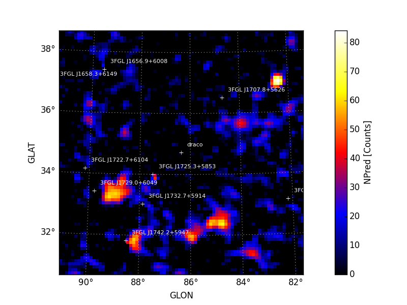
Maps are also written as both FITS and rendered image files to the analysis working directory. All output files are prepended with the prefix argument. Sample images for sqrt_ts and npred generated by tsmap() are shown below. A colormap threshold for the sqrt_ts image is applied at 5 sigma with iscontours at 2 sigma intervals (3,5,7,9, ...) indicating values above this threshold.

Sqrt(TS)	NPred

Reference/API¶

GTAnalysis.tsmap(prefix=u'', **kwargs)

Generate a spatial TS map for a source component with properties defined by the model argument. The TS map will have the same geometry as the ROI. The output of this method is a dictionary containing Map objects with the TS and amplitude of the best-fit test source. By default this method will also save maps to FITS files and render them as image files.

This method uses a simplified likelihood fitting implementation that only fits for the normalization of the test source. Before running this method it is recommended to first optimize the ROI model (e.g. by running optimize()).

Parameters:	prefix (str) – Optional string that will be prepended to all output files (FITS and rendered images). model (dict) – Dictionary defining the properties of the test source. exclude (str or list of str) – Source or sources that will be removed from the model when computing the TS map. erange (list) – Restrict the analysis to an energy range (emin,emax) in log10(E/MeV) that is a subset of the analysis energy range. By default the full analysis energy range will be used. If either emin/emax are None then only an upper/lower bound on the energy range wil be applied. max_kernel_radius (float) – Set the maximum radius of the test source kernel. Using a smaller value will speed up the TS calculation at the loss of accuracy. The default value is 3 degrees. make_plots (bool) – Write image files. make_fits (bool) – Write FITS files.
Returns:	maps – A dictionary containing the `Map` objects for TS and source amplitude.
Return type:	dict

Residual Map¶

residmap() calculates the residual between smoothed data and model maps. Whereas tsmap() fits for positive excesses with respect to the current model, residmap() is sensitive to both positive and negative residuals and therefore can be useful for assessing the model goodness-of-fit. The significance of the data/model residual at map position (i, j) is given by

\[\sigma_{ij}^2 = 2 \mathrm{sgn}(\tilde{n}_{ij} - \tilde{m}_{ij}) \left(\ln L_{P}(\tilde{n}_{ij},\tilde{n}_{ij}) - \ln L_{P}(\tilde{n}_{ij},\tilde{m}_{ij})\right)\]\[\mathrm{with} \quad \tilde{m}_{ij} = (m \ast k)_{ij} \quad \tilde{n}_{ij} = (n \ast k)_{ij} \quad \ln L_{P}(n,m) = n\ln(m) - m\]

where n and m are the data and model maps and k is the convolution kernel. The spatial and spectral properties of the convolution kernel are defined with the model argument. All source models are supported as well as a gaussian kernel (defined by setting SpatialModel to Gaussian). The following examples illustrate how to run the method with different spatial kernels.

# Generate residual map for a Gaussian kernel with Index=2.0 and
# radius (R_68) of 0.3 degrees
model = {'Index' : 2.0,
         'SpatialModel' : 'Gaussian', 'SpatialWidth' : 0.3 }
maps = gta.residmap('fit1',model=model)

# Generate residual map for a power-law point source with Index=2.0 for
# E > 3.16 GeV
model = {'Index' : 2.0, 'SpatialModel' : 'PointSource'}
maps = gta.residmap('fit1_emin35',model=model,erange=[3.5,None])

# Generate residual maps for a power-law point source with Index=1.5, 2.0, and 2.5
model={'SpatialModel' : 'PointSource'}
maps = []
for index in [1.5,2.0,2.5]:
    model['Index'] = index
    maps += [gta.residmap('fit1',model=model)]

residmap() returns a maps dictionary containing Map representations of the residual significance and amplitude as well as the smoothed data and model maps. The contents of the output dictionary are described in the following table.

Key	Type	Description
sigma	`Map`	Residual significance in sigma.
excess	`Map`	Residual amplitude in counts.
data	`Map`	Smoothed counts map.
model	`Map`	Smoothed model map.
files	dict	File paths of the FITS image files generated by this method.
src_dict	dict	Source dictionary with the properties of the convolution kernel.

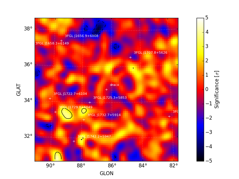
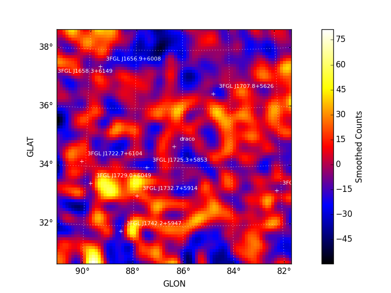
Maps are also written as both FITS and rendered image files to the analysis working directory. All output files are prepended with the prefix argument. Sample images for sigma and excess generated by tsmap() are shown below. A colormap threshold for the sigma image is applied at both -5 and 5 sigma with iscontours at 2 sigma intervals (-5, -3, 3, 5, 7, 9, ...) indicating values above and below this threshold.

Sigma	Excess Counts

Reference/API¶

GTAnalysis.residmap(prefix='', **kwargs)

Generate 2-D spatial residual maps using the current ROI model and the convolution kernel defined with the model argument.

Parameters:	prefix (str) – String that will be prefixed to the output residual map files. model (dict) – Dictionary defining the properties of the convolution kernel. exclude (str or list of str) – Source or sources that will be removed from the model when computing the residual map. erange (list) – Restrict the analysis to an energy range (emin,emax) in log10(E/MeV) that is a subset of the analysis energy range. By default the full analysis energy range will be used. If either emin/emax are None then only an upper/lower bound on the energy range wil be applied. make_plots (bool) – Write image files. make_fits (bool) – Write FITS files.
Returns:	maps – A dictionary containing the `Map` objects for the residual significance and amplitude.
Return type:	dict

TS Cube¶

Warning

This method is experimental and is not supported by the current public release of the Fermi STs.

GTAnalysis.tscube(prefix=u'', **kwargs)

Generate a spatial TS map for a source component with properties defined by the model argument. This method uses the gttscube ST application for source fitting and will simultaneously fit the test source normalization as well as the normalizations of any background components that are currently free. The output of this method is a dictionary containing Map objects with the TS and amplitude of the best-fit test source. By default this method will also save maps to FITS files and render them as image files.

Parameters:	prefix (str) – Optional string that will be prepended to all output files (FITS and rendered images). model (dict) – Dictionary defining the properties of the test source. do_sed (bool) – Compute the energy bin-by-bin fits. nnorm (int) – Number of points in the likelihood v. normalization scan. norm_sigma (float) – Number of sigma to use for the scan range. tol (float) – Critetia for fit convergence (estimated vertical distance to min < tol ). tol_type (int) – Absoulte (0) or relative (1) criteria for convergence. max_iter (int) – Maximum number of iterations for the Newton’s method fitter remake_test_source (bool) – If true, recomputes the test source image (otherwise just shifts it) st_scan_level (int) – make_plots (bool) – Write image files. make_fits (bool) – Write FITS files.
Returns:	maps – A dictionary containing the `Map` objects for TS and source amplitude.
Return type:	dict

Source Finding¶

Warning

This method is experimental and still under development. API changes are likely to occur in future releases.

find_sources() is an iterative source-finding algorithm that uses peak detection on the TS map to find the locations of new sources.

GTAnalysis.find_sources(prefix='', **kwargs)[source]

An iterative source-finding algorithm.

Parameters:

model (dict) – Dictionary defining the properties of the test source. This is the model that will be used for generating TS maps.
sqrt_ts_threshold (float) – Source threshold in sqrt(TS). Only peaks with sqrt(TS) exceeding this threshold will be used as seeds for new sources.
min_separation (float) – Minimum separation in degrees of sources detected in each iteration. The source finder will look for the maximum peak in the TS map within a circular region of this radius.
max_iter (int) – Maximum number of source finding iterations. The source finder will continue adding sources until no additional peaks are found or the number of iterations exceeds this number.
sources_per_iter (int) – Maximum number of sources that will be added in each iteration. If the number of detected peaks in a given iteration is larger than this number, only the N peaks with the largest TS will be used as seeds for the current iteration.
tsmap_fitter (str) –
Set the method used internally for generating TS maps. Valid options:
- tsmap
- tscube
tsmap (dict) – Keyword arguments dictionary for tsmap method.
tscube (dict) – Keyword arguments dictionary for tscube method.